Seeing (data) is believing (data)
4. Variance and distributions
We’ve seen the use of means and medians, but could still get fooled by these one number summaries. You may have experienced this with concert tickets. A seller might list the average ticket price of a concert of 20 USD then on the website you see the best seats are actually 100 USD with terrible seats at 5 USD. The seller could easily change the number and price of tickets in all sorts of ways to make the average seem affordable. That’s why understanding the spread of ticket prices, or the spread of whatever data we might be interested in, can help us be smarter buyers.
In the world of statistics, two important measures called variance and standard deviation help us understand how data points differ from the average and how much the data is spread from the average.
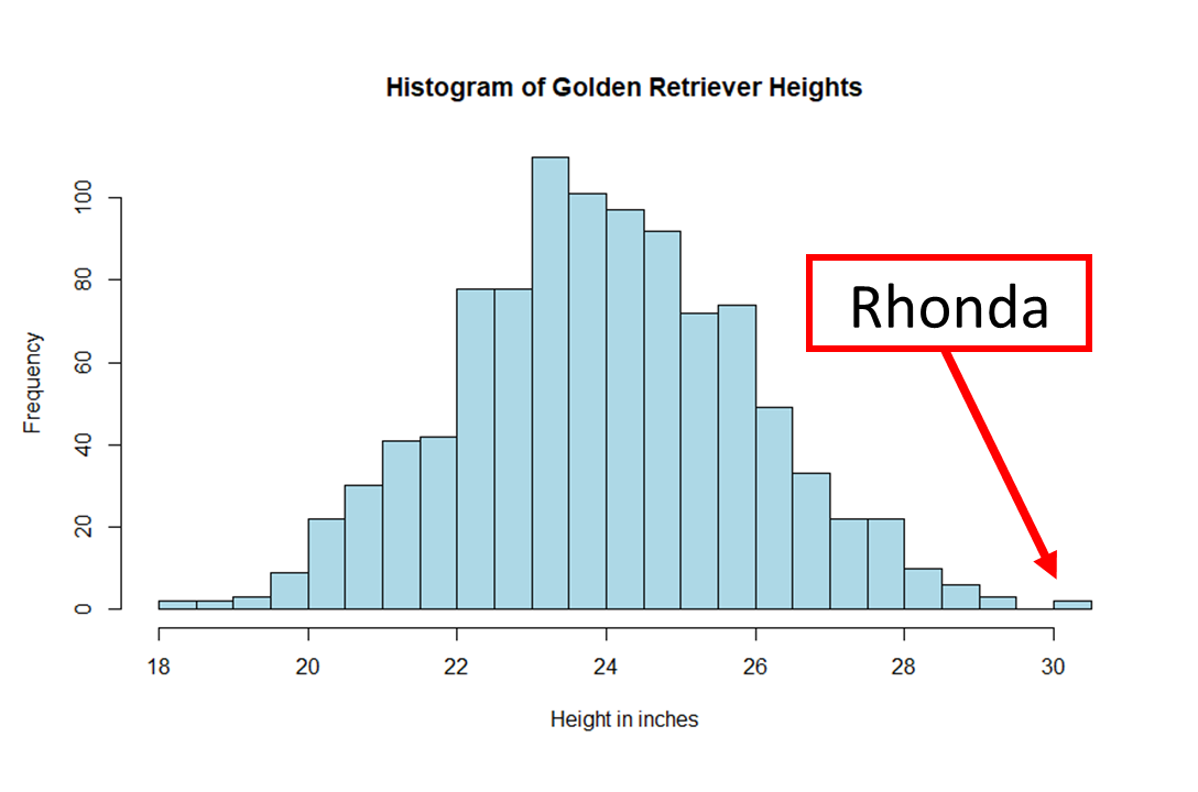
Let’s think about Rhonda’s 30 inch height again.
When we talk about variance, we’re talking about how much the individual heights of golden retrievers in our dataset differ from the average height of all golden retrievers. It helps us understand if the heights of the dogs are mostly similar or if there is a wide range of heights. Variance is calculated by taking the squared difference between each height and the average height, adding them up, and then dividing by the number of measurements in our sample.
For a Sample’s Variance:
Where:
- \(x_i\) represents each individual data point.
- \(\bar{x}\) is the mean of the sample.
- \(n\) is the total number of data points in the sample.
Example: Let’s calculate a made up sample of golden retriever height variance!
Imagine we have the following data of golden retriever heights:
\[2, 4, 6, 8, 10\]1. Calculate the mean (\(\bar{x}\)):
\(\bar{x}=\frac{2 + 4 + 6 + 8 + 10}{5} = 6\)
2. Subtract the mean and square the result for each data point:
\((2-6)^2 = 16\)
\((4-6)^2 = 4\)
\((6-6)^2 = 0\)
\((8-6)^2 = 4\)
\((10-6)^2 = 16\)
3. Calculate the average of those squared differences:
\(s^2=\frac{16 + 4 + 0 + 4 + 16}{5-1} = \frac{40}{4} = 10\)
The sample’s height variance \(s^2\) for the data set is \(10\). This is a decent amount of work doing these calculations by hand, so for data sets that have thousands or millions of data points, you can probably appreciate having a computer to help with these tasks!
Now, standard deviation is a measure that is easier to understand. It’s like the “average amount of difference” among the variation in a continuous variable. We can think of it as a typical or average distance that golden retriever heights deviate from the mean. To obtain standard deviation, you complete all the steps of calculating variance and then take the square root.
Calculate the standard deviation ($s$):
\(s = \sqrt{10} \approx 3.16\)
The standard deviation (\(s\)) for the data set is approximately \(3.16\). Standard deviation may also be abbreviated SD or STD in research and statistics.
Standard deviation spreads of continuous variables typically follow a similar bell-shaped curve pattern. By knowing the standard deviation and mean of golden retrievers’ heights, we can understand a lot about the spread of height data. If the average height of golden retrievers is 24 inches and the standard deviation is 2 inches, we can expect most golden retrievers to have heights that range from 22 to 26 inches. In a bell shaped curve, we can use the mean and standard deviation to figure out the proportion of the sample that have certain heights.
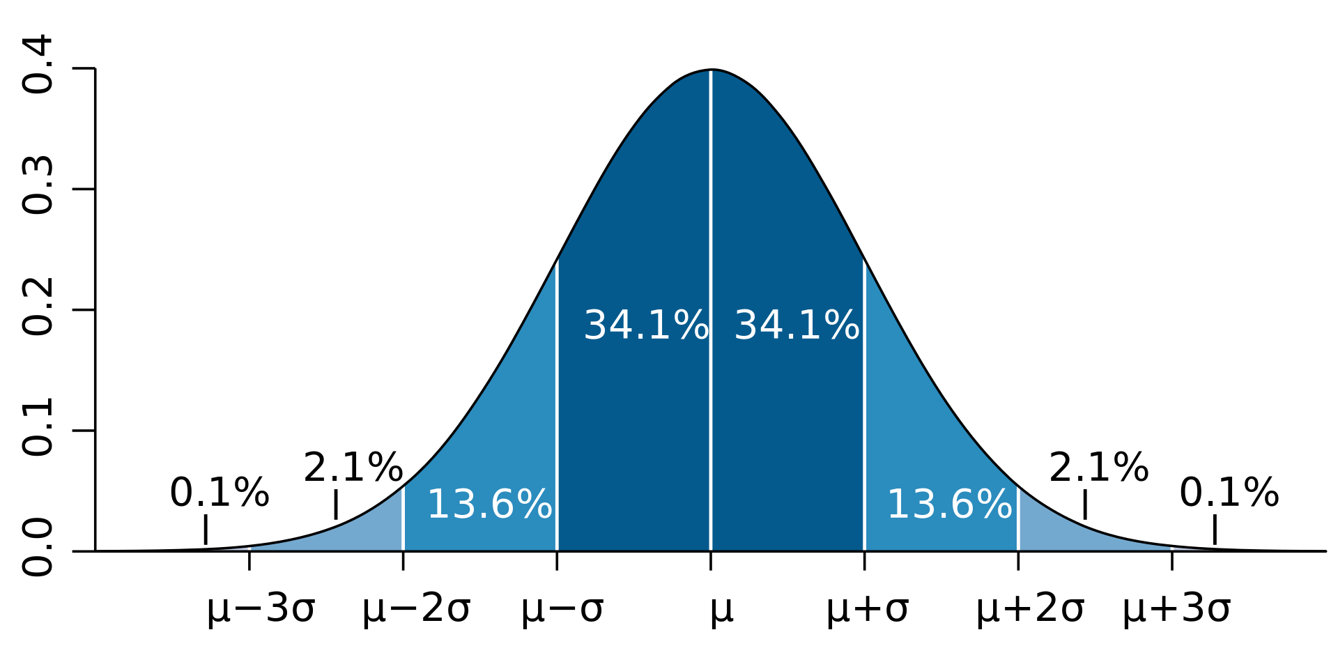
Figure by Ainali on Wikipedia- CC-BY-SA 3.0
Based on the curves above, we can see that the likelihood of a golden retriever being Rhonda’s height is very low! In fact, she is past the 3 standard deviations mark, so the probability of randomly finding a golden retriever with her height is around 0.1% !
Understanding the variance and standard deviation of Golden Retriever heights can be helpful for different reasons. Breeders can use standard deviations for expectations of a dog breed’s heights. For veterinarians, standard deviation helps determine if a Golden Retriever’s height is within a normal range for its age and breed, which can be important for monitoring their health. For us, standard deviation lets us know Rhonda is amazing and we should give her too many toys.
For more about visualizing data curves, check out this video from Khan Academy.
We could get an idea of what a sample of data looks like based on means and standard deviations alone, but it can be easier to fully visualize what our data looks like based on its spread, or distribution.
More visualization here.
In many cases of how data is distributed, the pattern follows a concept called a “normal distribution”. Normal distributions are patterns that often appear in data and we have seen one already! They have a special bell-shaped curve, with the highest point in the middle. In a normal distribution, data is evenly spread around the average, with most values near the middle and fewer values as we move away from the average. Many real-world things, like heights for golden retrievers or humans, tend to follow a normal distribution. Understanding normal distributions helps us make predictions and compare data.
There are cases when values for a variable we are interested in do not follow a “normal distribution”. Sometimes extreme values, or just the way a variable is, leads to skewed data distributions.
Skewness is a concept that helps us understand the shape and symmetry of data. When data is skewed, it means that it is not evenly or normally distributed. Skewed data distributions can be skewed to the left, where the longer tail is on the left side, or skewed to the right, where the longer tail is on the right side.
Skewness tells us if our data leans more towards one side or if it is balanced. Understanding skewness helps us recognize different patterns in data and interpret information accurately.
For more on skewness on curves, check out this video from Khan Academy.
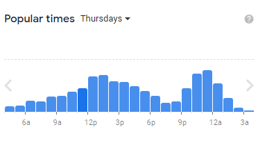
An example of a non-normal distribution is customer frequency on Thursdays at the McDonald’s on Time Square in New York, according to Google Maps as of 8-30-23. You can see there is a customer rush around lunch time and around dinner.
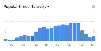
A distribution closer to normal is customer frequency on Saturdays at the McDonald’s on Time Square in New York, according to Google Maps as of 8-30-23. You can see there may be the first customer rush around lunch time but then the customer frequency continues to grow!
Histograms, like the two pictures above, are visual representations that help us understand the distribution of continuous data. Histograms display data in organized bars or columns on a graph. Each bar represents a range of values, and the height of the bar shows how many data points fall within that range. Histograms allow us to see patterns, such as the most common values or any outliers. They help us understand the shape of the data, whether it is symmetric, skewed, or has other unique characteristics. By using histograms, we can analyze and interpret data more easily, making it a valuable tool in understanding information visually.
If you want more info on creating histograms, check out this video by Khan Academy.
You can also play with distributions and how the median and mean are affected in the webapp below!
To summarize, variance and standard deviation help us measure how data points differ from the average and give us an idea of how our continuous data is spread. These measures are important tools in statistics that allow us to better understand and analyze data in many different fields and trends.
Variance and standard deviation can even help us be smarter shoppers and buyers (or visitors to restaurants in busy areas!). The spread of data is often the first step of interpreting data and is also useful for when you begin to analyze data.
If you’d like to play around with visualizing distributions, and other plots and statistics, you can play with the Wisconsin Fast Stats app which can give you sample data about plant baby leaf numbers (AKA cotyledons) by generation.
In statistics, variance and standard deviation are measures used to understand how much data points differ from the average and the overall spread of the data. They help us see if data points are close together or spread out, like the range of heights in dogs or prices of concert tickets.